Dynamics is the study of how objects move and respond to forces, and the techniques are used across many industries including aerospace, automotive, civil and more. When designing an engineering system, it can be expensive and unrealistic to go directly from a basic set of equations to a fully complete, working product. Simulation is a tool that is frequently used to model systems and test and validate algorithms or designs early in the design process.

In this article, I will cover simulating dynamic motion using C++, a programming language often used for it’s performance. For simple simulations, higher level languages may be suitable, but as the fidelity increases, so does the computation requirements.

This tutorial will start with defining a simple yet commonly used dynamics model, the 2nd order mass-spring damper system. Armed with the equations of motion, I will then design a C++ simulation of the system dynamics. Let’s jump in!

The Mass-Spring Damper System

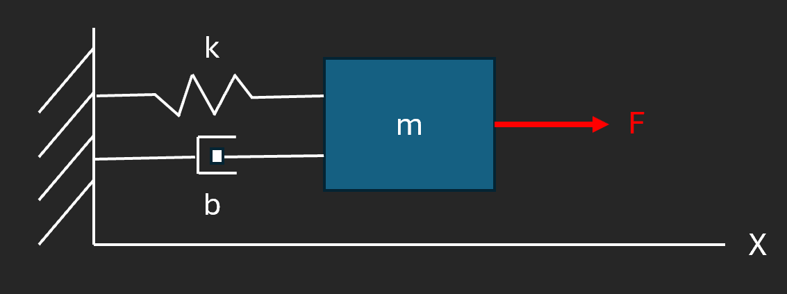
The first step in any simulation is modeling the system. Typically, models start simple and are scaled to higher levels of fidelity as the design matures. For our system, imagine we have a basic spring-mass damper system that moves in a single dimension.

The spring has a stiffness constant, k, and the damper has a damping constant, b. The test block, with mass m, is attached to the end and can move along the x-axis. Assume an external force can be applied along the direction of movement, denoted in the diagram above by F.

To model this system, start with a free body diagram of the test block and the forces that act on it. Since spring forces are proportional to the distance from equilibrium and damping forces are proportional to the blocks velocity, our free body diagram can be written as:

This is making the assumption that equilibrium is at x = 0. Next, using Newton’s 2nd law, we can write out the equations of motion of the block. This 2nd order equation governs how the dynamics will evolve over time in response to the forces applied.

In the study of differential equations, there are often no closed form solutions, especially to higher order systems. Fortunately, state space system modeling gives us a tool for handling this. We can convert any arbitrary nth order dynamic equation into a system of n first order differential equations. Once the equations are in this form. we have a number of numerical techniques available to solve this problem.

Since our mass-spring damper system is 2nd order, we can convert it into a system of 2 first order differential equations of the form

The first term (Ax) represents the free dynamics, or the system response to the initial conditions, while the second term (f), represents the forced response. For a more detailed description of state space system modeling, see this page. We can define our state space, x, as

which is the 1D position and velocity of the block. To get the state space model, we can differentiate our state and plug in the equation of motion.

Finally, let’s refactor the right hand side of the equation to match the generic form of the state space system from before.

The model is now in a form that we can simulate.

Simulation in C++

Now that we have our equations of motion, we can turn our attention to the software implementation. Since this system represents a differential equation, we need a numerical integration scheme, along with a set of initial conditions to propagate the system dynamics over time.

For now, we will use a simple 1st order Euler numerical integration method. Higher precision methods do exist, make sure to check back on this blog in the future for a post on other techniques. Euler’s method is given by:

Pretty simple right? The state at a given iteration, k+1, is equal to the state at the previous iteration, k, plus the derivative at iteration k, multiplied by the time interval from k to k+1. Technically, this doesn’t have to be the time interval, it could be any interval of integration. However, since we are looking at dynamics over time, we will keep it this way for simplicity.

One final piece of information we need to simulate this system is a set of initial conditions for the state. As you will see in the unforced case shortly, these initial conditions are key to determining how the state will evolve over time.

At this point we now have our dynamics model, our numerical integration scheme, and the knowledge that we need to included initial conditions, let’s move to simulating these dynamics in C++.

Typically, I would recommend setting up a local development environment, but for simplicity here, I will use an online C++ compiler so that we can focus on just the software part. I prefer using this one, but anything that allows you to run the code below quickly should do.

One final thing to note is that to avoid package dependencies that could make running this difficult for you, I have implemented this using only the C++ standard library with a set of custom structs representing 2D vectors and matrices, and a few utility functions needed for the algorithm. In practice, using a more generic and powerful Linear Algebra library, for example like Eigen, can make this a much simpler process.

#include <iostream>
#include <vector>

// Define a 2D vector
struct vec2 {
    double v1;
    double v2;
};

// Define a 2D Matrix
struct mat2 {
    double v11;
    double v12;
    double v21;
    double v22;
};

// Function to multiply a 2D matrix by a 2D vector
vec2 multiply(mat2 m, vec2 v) {
    vec2 out = {m.v11*v.v1 + m.v12*v.v2, m.v21*v.v1 + m.v22*v.v2};
    return out;
}

// Function to multiply a 2D vector by a scalar
vec2 multiply(vec2 v, double s) {
    vec2 out = {v.v1*s, v.v2*s};
    return out;
}

// Function to add two 2D vectors
vec2 add(vec2 v1, vec2 v2) {
    vec2 out = {v1.v1 + v2.v1, v1.v2 + v2.v2};
    return out;
}

/**
 * Dynamics Model class
 * 
 * This class stores the dynamics model parameters,
 * state and contains functions for propagating the
 * system dynamics in response to a forcing function.
 */
class dynamicSystem {
  public:
    // c'tor - sets the system parameters
    dynamicSystem(const vec2& x0, const double m, const double k, const double b, const double t) :
        x_(x0), m_(m), k_(k), b_(b), t_(t) { }
        
    // Function to get the State
    vec2 getState() const { return x_; }
        
    // Propagate dynamics to some time t, with a constant force applied
    void propagateDynamics(const double t, const double F) {
        // Compute Delta time
        double dt = t - t_;
        
        // Define A matrix
        mat2 A = {0.0, 1.0, -k_/m_, -b_/m_};
        
        // Define Forcing function
        vec2 forcing = {0.0, F/m_};
        
        // Define State derivative, xDot
        vec2 Ax = multiply(A, x_);
        vec2 xDot = add(Ax, forcing);
        
        // Propagate dynamics
        vec2 dx = multiply(xDot, dt);
        x_ = add(x_, dx);
        
        // Update time
        t_ = t;
    }
    
  private:
    // System state vector
    vec2 x_;
    
    // System mass (kg)
    double m_;
    
    // Spring constant (N/m)
    double k_;
    
    // Damping Constant (Ns/m)
    double b_;
    
    // System time (s)
    double t_;
};

int main()
{
    // Define the model parameters
    double k = 1.0;
    double b = 0.3;
    double m = 3.0;
    
    // Define our initial state
    vec2 x0 = {2.0, 0.0}; 
    
    // Define a vector of times
    std::vector<double> times{0.0};
    for (int i = 1; i < 101; i++) {
        times.push_back(times.back() + 0.1);
    }
    
    // Construct the dynamics model
    dynamicSystem sys(x0, m, k, b, times[0]);

    // Loop over times, propagate dynamics with no force and print states
    for (int i = 0; i < times.size(); i++) {
        sys.propagateDynamics(times[i], 0.0);
        vec2 stateCurr = sys.getState();
        std::cout << times[i] << "," << stateCurr.v1 << "," << stateCurr.v2 << std::endl;
    }
    return 0;
}

The time, position and velocity are printed to the terminal. Collecting the data and plotting it yields the results:

You have now run a dynamic simulation of the system! I recommend testing out different system parameters (mass, spring/damping constants and initial conditions) to see how the dynamics change. You could also experiment with adding external forces. To generate the plots, simply collect the output from the terminal, save it in a file called “Data.txt”, and run this Python script:

## Plot the dynamic simulation results
import pandas as pd
import matplotlib.pyplot as plt

# Load the data from the text file
file_path = 'Data.txt'
data = pd.read_csv(file_path, header=None, names=['time', 'x', 'y'])

# Create a figure with two stacked subplots
fig, axs = plt.subplots(2, 1, figsize=(10, 8), sharex=True)

# Plot time vs position on the top subplot
axs[0].plot(data['time'], data['x'], color='blue')
axs[0].set_title('Position vs Time')
axs[0].set_ylabel('Position (m)')
axs[0].grid()

# Plot time vs velocity on the bottom subplot
axs[1].plot(data['time'], data['y'], color='red')
axs[1].set_title('Velocity vs Time')
axs[1].set_ylabel('Velocity (m/s)')
axs[1].set_xlabel('Time (s)')
axs[1].grid()

# Format Plot
plt.tight_layout()
plt.show()

Conclusion

In this post, we covered how to simulate system dynamics in C++. This approach can be used on any arbitrary system that can be modeled in state space space form, and is a highly effective means of understanding a system in a quick, low cost way. For systems of the complexity in this article, Matlab/Python/etc. may be an appropriate tool, however as model complexity grows, the benefits of C++ performance become more important.

I hope you enjoyed this post and learned something new. Make sure to check back soon for more posts and algorithm implementations. Happy coding!

-Parker