Derivatives measure the rate of change of a quantity and are used across all fields of engineering. Whether you are trying to understand the dynamic motion of robots, modeling flow rates, or any other number of applications, being able to estimate derivates numerically, especially when they cannot be directly measured, is a crucial skills for any engineer. In this post, we cover numerical methods for differentiation – aka, how to estimate derivates.
Forward/Backward Difference
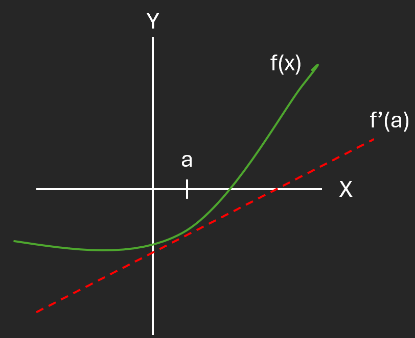
Estimating derivatives involves finding the slope of the tangent line to a curve at a given point. For example, if we have a curve, f(x), then the derivative at the point x = a can be found by drawing a tangent line (the red dashed line below) at this point and calculating the slope.

For many functions, the tangent line will only provide a good approximation of the derivative in a small neighborhood around the point, x = a. If you move too far in either direction, the tangent line will change enough that you would likely need to calculate a new slope. One of the biggest challenges in implementing a numerical differentiation algorithm on real data is choosing an appropriate window size in which the assumptions made about the derivative are still valid.
Let’s assume, you are sitting at x = a and take a small step to the right by some distance h. Don’t worry too much about h, just know that it is small enough such that the derivative of f(x) changes a negligible amount. The slope of the tangent curve for this interval can easily be calculated by dividing the change in y values by the change in x values.

Congratulations, you just learned your first numerical differentiation algorithm! This particular algorithm is called a forward difference because we step forward in the positive direction from the point we want to evaluate the derivative at. We could just have easily stepped in the opposite direction, and used what we refer to as a backwards difference instead.

To implement either a forward or backward difference algorithm, simply iterate over your x evaluation points, calculating the derivative as you go. Here is some Python code that does this for a given function, f(x) = sin(x).
# Forward/Backward Difference Algorithms
import matplotlib.pyplot as plt
import numpy as np

# Define a step size interval
dx = 0.5

# Assume the target function is f(x) = sin(x). Define a function to evaluate f(x) at
# a given point.
def f(x):
    return np.sin(x)

# Create a vector containing data points of the true derivative of the target function
# which is given by f'(x) = cos(x). This will be used to characterize our algorithm
# performance.
x = np.arange(0, 3 * np.pi, dx)
fPrimeXTruth = np.cos(x)

# Initialize vectors of derivatives to be filled in by forward/backward difference
fPrimeXBackward = np.zeros_like(fPrimeXTruth)
fPrimeXForward = np.zeros_like(fPrimeXTruth)

# Loop over x values and calculate derivative using both methods
# At the first step, the backward difference cannot be calculated
# At the final step, the forward difference cannot be calculated
for i in range(len(x)):
    # Perform backward difference if not at the first point
    if i != 0:
        fPrimeXBackward[i] = (f(x[i]) - f(x[i-1])) / (x[i] - x[i-1])

    # Perform forward difference if not at the last point
    if i != len(x)-1:
        fPrimeXForward[i] = (f(x[i+1]) - f(x[i])) / (x[i+1] - x[i])

# Set the starting point of the backward difference equal to the second point and the
# final point of the forward difference to the second to last point. This approach is often
# used to smooth out the endpoints of the derivative estimate.
fPrimeXBackward[0] = fPrimeXBackward[1]
fPrimeXForward[-1] = fPrimeXForward[-2]

# Plot Results
plt.plot(x, fPrimeXTruth, label = "Truth")
plt.plot(x, fPrimeXBackward, label = "Backward Difference")
plt.plot(x, fPrimeXForward, label = "Forward Difference")
plt.title("Forward/Backwards Finite Difference, Step Size = " + str(dx))
plt.xlabel("x")
plt.ylabel("f'(x)")
plt.legend(loc='upper right')
plt.grid()
plt.show()
Running this code results in the following plot:

Notice that while our approximation is not bad, it definitely leaves something to be desired. In this case, the step size was set to 0.5, but this was likely way too large to generate a reasonable estimate. Let’s shrink this down and see what happens when it gets smaller.

Shrinking the step size down by a factor of 10, results in a derivative that is now almost a perfect approximation! If you continued to shrink the interval of each step, the estimate would continue to improve. Unfortunately, making this change also requires 10x the number of iterations to run.
This example is a good illustration of the challenge faced by the algorithm designer – balancing the accuracy of the estimate with the computational cost of running the algorithm. For a simple example like this one, the additional cost may be negligible. For more complex functions over longer intervals however, this can quickly get out of hand and motivates the need for higher order approaches which can achieve better performance with larger step sizes.
Central Difference
The forward and backward difference algorithms discussed above are what we call 1st order algorithms, because they can estimate a derivative to a first order approximation by fitting a straight line between two points. One of the drawbacks of these two approaches however is that they implicitly estimate the derivative at the start or the end of the interval, however the estimate is really the most accurate in the middle.
The Central Difference algorithm is another 1st order approach, however it leverages points in both the forwards and backwards direction so that it is estimating a derivative at the center of the interval, thereby increasing the accuracy. The Central Difference equation is given by:

We are still fitting a straight line between points, but now using points on either side of the evaluation point. Let’s recreate the Python code from before, but this time using a Central Difference algorithm instead:
# Central Difference Algorithms
import matplotlib.pyplot as plt
import numpy as np

# Define a step size interval
dx = 0.5

# Assume the target function is f(x) = sin(x). Define a function to evaluate f(x) at
# a given point.
def f(x):
    return np.sin(x)

# Create a vector containing data points of the true derivative of the target function
# which is given by f'(x) = cos(x). This will be used to characterize our algorithm
# performance.
x = np.arange(0, 3 * np.pi, dx)
fPrimeXTruth = np.cos(x)

# Initialize vectors of derivatives to be filled in by central difference
fPrimeXCentral = np.zeros_like(fPrimeXTruth)

# Loop over x values and calculate derivative
# At the first and last step, the central difference cannot be calculated
for i in range(len(x)):
    # Perform central difference if not at the first/last point
    if i != 0 and i != len(x)-1:
        fPrimeXCentral[i] = (f(x[i+1]) - f(x[i-1])) / (x[i+1] - x[i-1])

# Set the starting point of the central difference equal to the second point and the
# final point of the central difference to the second to last point. This approach is often
# used to smooth out the endpoints of the derivative estimate.
fPrimeXCentral[0] = fPrimeXCentral[1]
fPrimeXCentral[-1] = fPrimeXCentral[-2]

# Plot Results
plt.plot(x, fPrimeXTruth, label = "Truth")
plt.plot(x, fPrimeXCentral, label = "Central Difference")
plt.title("Central Finite Difference, Step Size = " + str(dx))
plt.xlabel("x")
plt.ylabel("f'(x)")
plt.legend(loc='upper right')
plt.grid()
plt.show()
Try running this code and you should get the following plot:

Notice how much better this performs than either the forward or backward difference when the step size = 0.5! In practice, this means you can achieve vastly improved performance overall with many less iterations required. Just like before, you could continue to decrease the step size to get improved performance, but you would likely need many less steps to achieve the same results as the other methods we have covered so far.
Higher Order Derivatives
As you might imagine, we sometimes need not just the 1st order derivative of a function, but also the 2nd order and beyond. One approach that is often used to approximate second order derivatives is re-applying the central difference formula to estimate the 2nd derivative:

You are probably wondering why we are evaluating this expression at 1/2 h now, and that is a completely valid question. Remember that we can choose any value for h that makes sense for our problem and as you will see in just a second, using the 1/2 term will simplify our final expression greatly. From our definition of the central difference, we know that

When we plug these terms into our expression for the second derivative and simplify, we get:

This expression is extremely powerful because it only depends on the function, f(x) – this means that we can estimate the 2nd derivative without first estimating the 1st derivative! Let’s write some Python code and see how this works in practice.
# 2nd Order Difference Algorithm
import matplotlib.pyplot as plt
import numpy as np

# Define a step size interval
dx = 0.5

# Assume the target function is f(x) = sin(x). Define a function to evaluate f(x) at
# a given point.
def f(x):
    return np.sin(x)

# Create a vector containing data points of the true 2nd derivative of the target function
# which is given by f''(x) = -sin(x). This will be used to characterize our algorithm
# performance.
x = np.arange(0, 3 * np.pi, dx)
fPrimePrimeXTruth = -np.sin(x)

# Initialize vectors of 2nd derivatives to be filled in by the difference algorithm
fPrimePrimeX = np.zeros_like(fPrimePrimeXTruth)

# Loop over x values and calculate derivative
# At the first and last step, the difference cannot be calulated
for i in range(len(x)):
    # Perform 2nd order difference if not at the first/last point
    if i != 0 and i != len(x)-1:
        # Calculate the step size
        h = (x[i+1] - x[i-1]) / 2.0

        # Estimate the derivative
        fPrimePrimeX[i] = (f(x[i+1]) - 2*f(x[i]) + f(x[i-1])) / (h**2)

# Set the starting point of the central difference equal to the second point and the
# final point of the central difference to the second to last point. This approach is often
# used to smooth out the endpoints of the derivative estimate.
fPrimePrimeX[0] = fPrimePrimeX[1]
fPrimePrimeX[-1] = fPrimePrimeX[-2]

# Plot Results
plt.plot(x, fPrimePrimeXTruth, label = "Truth")
plt.plot(x, fPrimePrimeX, label = "2nd Order Difference")
plt.title("2nd Order Finite Difference, Step Size = " + str(dx))
plt.xlabel("x")
plt.ylabel("f''(x)")
plt.legend(loc='upper right')
plt.grid()
plt.show()
If you run this code for a few different step sizes, you can get the following results:

As you can see, this approach can give very good approximations of the 2nd derivative of a function. The same approach could be used to derive even higher order derivatives as well!
Conclusion
In this article, we covered a few of the most common numerical methods used for estimating first and second order derivatives. These techniques are extremely powerful and have applications in a wide number of fields.
I hope you enjoyed this tutorial, be sure to check out one of my other posts here and let me know what you think of this tutorial in the comments. Happy programming!
-Parker


