Few tools exist that are used as widely as linear regression. Whether it’s cutting edge machine learning or making predictions about sports outcomes based on historical data, linear regression touches nearly all industries and problem spaces. In this post, I will cover the theory behind linear regression and walk through a simple C++ implementation available in the Machine Learning Toolbox.

How Linear Regression Works

Linear regression is a supervised machine learning technique for findings a linear relationship between a set of independent variables and a dependent variable. It can be used for making future predictions about continuous variables from historical data.

There are two main models of linear regression: simple and multiple. The simple model is the equation of a straight line we all know and love:

the first term, b0, is the intercept and b1 is the slope. The “b” terms are what we refer to as the model weights or coefficients, while x1 is the independent variable, sometimes referred to as the predictor. y then, is the dependent variable. Linear regression is about using some set of training data, (x,y) pairs, to estimate the model weights. Once the model weights are set, we can make predictions about the independent variable y, given any input x.

Often, there is more than one independent variable that impacts the dependent variable. We can extend the simple model to allow for more independent variables, sometimes referred to as a multiple linear regression:

The next natural question is then, “how do we come up with the model weights”? The goal of linear regression is to minimize the error in our prediction, therefore it makes sense to define the model weights such that the resulting model minimizes the total residual error across all measurements.

This can be formulated as an optimization problem! While we could use a number of different cost functions to minimize, let’s use the sum of the square of the errors. The reason why will become clear shortly:

Notice that this is just the cost function used in Least Squares Estimation! The complete derivation of optimizing this cost function is outside the scope of this article, but since it is just the least squares problem, the solution becomes:

Where:

Each row of B corresponds to the model weights and is the vector we are solving for. Each row of X corresponds to the independent observations used to train the model. Notice the “1” in the first column, this allows us to formulate the entire linear model in matrix form, rather than using multiple matrices.

Each row of Y corresponds to the individual observations of the dependent variable in the training set. X and Y have m rows, and to avoid an under-determined least squares problem, m must be greater than or equal to the number of model weights, n.

Once we have solved the least squares regression, we can use the results to make predictions. In particular, the prediction of y, will be:

This expression can be used for both single predictions or a batch of predictions. Now that we have covered the theory behind linear regression, let’s cover a simple C++ software which uses the Eigen linear algebra library.

Linear Regression Example

For the complete algorithm implementation, see this page for the header file and this page for the source implementation. A common example of linear regression is predicting rent prices based on square footage. This problem can be represented as a simple model in which square footage is the independent variable and rent is the dependent variable.

Assume we have the following set of training data.

We can now use the Machine Learning Toolbox library to train a linear model on this data. The code to do this is below and can be found here.

/**
 * A Linear Regression example
 *
 * Problem statement: Given the table of square footage and rent data below,
 * train a linear regression model on the data and make predictions of rent
 * price given an apartment's square footage.
 *
 * Training Data
 * Square Footage = [500, 750, 1000, 1250, 1500, 1750]
 * Rent = [1000, 1300, 2200, 2400, 3150, 3400]
 *
 * Predictions:
 * Square Footage = 1100, Rent = ?
 * Square Footage = 1300, Rent = ?
 * Square Footage = 2000, Rent = ?
 */
#include "SupervisedLearning/Regression/LinearRegression.h"
#include <iostream>

int main() {
  // Create a simple linear regression
  LinearRegression lr;

  // Create a matrux of training data
  Eigen::Matrix<double, 6, 2> trainingData;
  trainingData << 500, 1000, 750, 1300, 1000, 2200, 1250, 2400, 1500, 3150,
      1750, 3400;

  // Add the data to the model and train
  lr.addTrainingData(trainingData);
  bool solveSuccess = lr.solveRegression();
  if (!solveSuccess) {
    std::cout << "Failed to solve regression. Terminating..." << std::endl;
    return 1;
  }

  // Print Model Weights
  Eigen::VectorXd predictorWeights = lr.getPredictorWeights();
  std::cout << "Linear Regression Predictor Weights:" << std::endl;
  for (int i = 0; i < predictorWeights.size(); i++) {
    std::cout << "    i = " << i << ", weight = " << predictorWeights(i)
              << std::endl;
  }

  // Create vector of square footage to make predictions on
  Eigen::Matrix<double, 3, 1> predictionValues;
  predictionValues << 1100, 1300, 2000;

  // Predict the rent
  auto maybePredictionResult = lr.predictBatch(predictionValues);
  std::cout << "Linear Regression Preictions:" << std::endl;
  if (maybePredictionResult.has_value()) {
    Eigen::VectorXd predictionResults = maybePredictionResult.value();
    for (int i = 0; i < predictionResults.size(); i++) {
      std::cout << "    (x,y) = (" << predictionValues(i) << ", "
                << predictionResults(i) << ")" << std::endl;
    }
  } else {
    std::cout << "Failed to make predictions. Terminating..." << std::endl;
    return 1;
  }
  return 0;
}

Running this code gives the following result:

Linear Regression Predictor Weights:
    i = 0, weight = -40.4762
    i = 1, weight = 2.02857
Linear Regression Predictions:
    (x,y) = (1100, 2190.95)
    (x,y) = (1300, 2596.67)
    (x,y) = (2000, 4016.67)

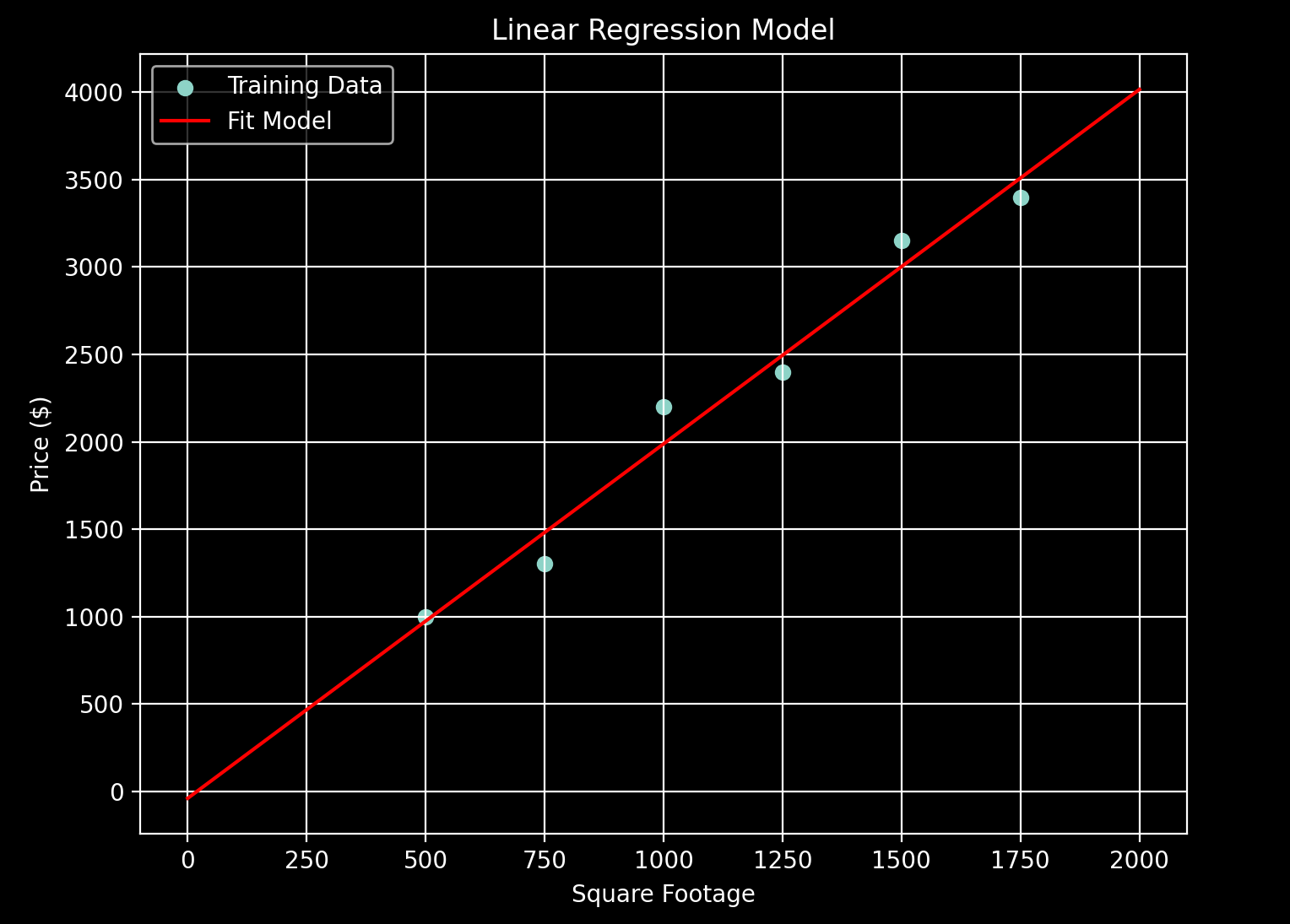
We can update our training data figure from above with a line given the model weights above as the y intercept (i = 0) and the slope (i = 1). The resulting model curve is:

Conclusion

I hope you enjoyed this tutorial on Linear Regression. In this post, we covered the theory behind the technique and created a simple example to showcase it. I recommend playing around with the code to build your regressor and experimenting with different models.

Make sure to check back soon another post and happy coding!

-Parker