Engineering problems often involve finding the roots of a given function. In controls, we use root-finding to determine equilibrium points of a system. Graphics engineers use these techniques for finding intersections between objects. And there are so many more applications for this important class of techniques. In today’s post, I will be covering several of the most popular bracketing methods for solving root finding problems.

Bracketing Methods

Bracketing methods are a class of techniques which involve selecting initial lower and upper bounds that “bracket” your solution and iteratively narrowing your bracket size around the solution until you have achieved some convergence criterion. The convergence criterion let’s you say “this is close enough to the solution” and we can stop running the algorithm.

Before we dive into the methods, you should first gain some insight into the structure of the problem to understand why bracketing methods even work. Let’s say we have a parabola and want to find the minimum point, something we do often (albeit on typically higher dimension and more complex surfaces) in optimization.

Intuitively, how might you find the minimum? In the case of the parabola, we known that either end always increases. This means that there must be some X value somewhere in the proverbial middle, such that the Y value is lower than at any other point. If you are sitting at that point and move in either direction, you will be increasing.

I made a big assumption in the above statement – that there was a single global minimum in the function. Real world optimization problems often involve functions with many local minimums and sometimes we are trying to find these, but other times we need to design algorithms that find the global minimum. For now, we will roll with our assumption of the single global minimum for simplicity.

Let’s say you know the minimum of the function is somewhere around X = 0, but you aren’t really sure exactly where. Bracketing methods involve selecting some safe upper and lower bound so that you are confident that the solution falls inside the bounds. If the solution falls outside the bounds, a bracketing method will converge to a result that is not the global minimum and nobody wants that!

Once we have a good starting point, the next step in a bracketing method is to push the bounds inwards, ever closer towards the minimum, until we’ve converged to a solution. We typically define a tolerance, the size of the interval, we are happy with to say that our solution has converged. Once the size of bounds are less than the convergence criteria, we can be confident the error in our solution will be within the tolerance.

Choosing a tolerance is a bit of an art. As an algorithm designer, you are constantly toeing the line between accuracy and speed. Typically, as the tolerance shrinks, the number of iterations of an algorithm required to achieve the convergence criteria goes up, hence leading to longer run times.

Ok, so can we dive into some algorithms now? Not quite – I haven’t mentioned anything yet about how we turn a minimization problem into a root finding problem, which is all about finding the zeros of a function.

At the minimum point, it stands to reason that the curve will be flat and hence the derivative equal to zero. In our parabola example above, if you take a small step to the left in the negative X direction, the slope is downwards and the derivative will be negative. A step to the right will have the opposite effect, and the derivative will be positive.

Another way to look at a minimization problem is not finding where the curve reaches it’s minimum value, but instead where the derivative function crosses 0! This approach often simplifies our algorithms and turns the problem into root finding. We can re-formulate our parabola minimization problem above as finding the roots, or zeros, of it’s derivative, a straight line.

Now that you understand the basic premise of bracketing methods, let’s go over a few of the most common ones.

Graphical Methods

Graphical methods are exactly like they sound – take a look at the graph and select the minimum, or in the root finding case, where the derivative crosses zero. These methods are usually good for simpler problems that can be visualized, but may be more difficult on more complex, multi-dimensional surfaces.

Computer software can often make graphical methods more tractable. For example, in Matlab or Python, you can generate a curve or surface and point and click to find the minimum. For some problems, this approach might be sufficient and is certainly the fastest way to a solution.

Personally, if I have a low dimension problem that requires root-finding, I love using graphical methods as a way of selecting reasonable starting bounds and then using one of the methods below to find a more precise minimum.

Bisection Method

The bisection method is fairly straightforward and intuitive, but is extremely powerful. Imagine you have no idea what function we are trying to find the roots for, but I give you the initial upper and lower bounds of the bracket. What if I asked you to guess where the root is in that interval?

You’d probably choose the mid-point, and that would be a totally reasonable approach with no other information available! This is exactly the premise behind the bisection method. Remember that in root finding, we try to find the zeros, or the point the curve crosses from negative to positive. (or the opposite for a decreasing derivative function).

To start, let’s grab the value of the curve at each of our initial bounds. Let’s say the lower bound has a value of -3 and the upper bound has a value of +5.

A reasonable initial guess of the root might be in the middle of the interval which we can get by adding the upper and lower bounds and dividing by 2. The mid-point is at X = (5 + (-3)) / 2 = 1. Since we are trying to find the point where the curve equals 0, but it equals 1 at this point, we know we haven’t yet found our root.

Next, we need to shrink this interval down and try again. Intuitively, we could either shift the lower bound or upper bound to the midpoint and consider the new interval, but we need to be careful that we choose to move the bound that keeps the zero inside the new interval. How do we do this?

Recall that the zero is where curve changes sign. We want our lower and upper bounds to ALWAYS have a different sign! This makes it really easy for us to choose which bound to move. Simply evaluate the midpoint and move the bound that has the same sign. For example, since the Y value of our midpoint is 1, this has the same sign as the upper bound, therefore we know it is still to the right of the solution, and hence we can move our upper bound inwards.

That makes sense, but how do we check this in software? We can do this multiplying the value of our function at the midpoint with the lower and upper bounds and checking the sign of the result. If the result is positive, we know the signs were the same and thus we can move the associated bound.

Now that we have our new bounds, we repeat until we find the solution. The midpoint of the new interval is at X = (1 + (-3)) / 2 = -1. We can evaluate the curve at this point and find that the Y value is equal to -1. Since this shares the same sign as the lower bound, we can shift our lower bound to this point. Are you starting to get the idea?

We don’t have a solution yet, so let’s keep going. The next midpoint of our reduced interval is at X = (1 – (-1)) / 2 = 0. At this point, our Y value is equal to 0 and we have found the solution! Congratulations, our bisection algorithm has converged. In practice, we rarely get the exact solution, but as long as we get to some value less than our tolerance, we can call it a solution.

We also don’t always know exactly what the truth is or if our derivative function is perfect and so we typically define our tolerance in reference to the size of our interval as this provides an upper bound on the error.

Pretty simple right? The larger your starting interval, typically the more steps you will need to take to converge. Now that you understand the algorithm, let’s write some code to solve this problem! Try changing the function and seeing what happens!

# Bisection Method Python Code Example
# Assume you want to minimize a parabola with the equation y = (1/2) * x^2 + 4
# The derivative is equal to y' = x

# A function to evaluate the derivative (y') at a given x value
def f(x):
    return x
    
# Define Initial Bounds
lowerBound = -3.0
upperBound = 5.0

# Define Convergence Criteria
eps = 1.0e-3

# Loop until the solution is found
i = 0
root = lowerBound # initialize
while (upperBound - lowerBound) > eps:
    # Increment the iteration counter
    i += 1
    
    # Print Iteration Status
    print("Iteration ", i, ", Lower Bound = ", lowerBound, ", upperBound = ", upperBound)
    
    # Get the midpoint
    root = (upperBound + lowerBound) / 2.0

    # Check for an exact solution
    if f(root) == 0.0:
        break
    
    # Check which bound to shift
    # Since we want the new bound to have the same sign as 
    # the one it is replacing, we can say that the product 
    # must be positive
    if f(lowerBound) * f(root) > 0:
        lowerBound = root
    else:
        upperBound = root
        
# Print Solution
print("Found solution at X = ", root)

False Position Method

The bisection method described above is easy to implement and makes sense, but it’s not always ideal. What if we have a large interval and need to run it many times? What if there was a way to take advantage of the information we have so that rather than blindly choosing the midpoint, we make a more intelligent guess of the root? The false position method allows us to do this.

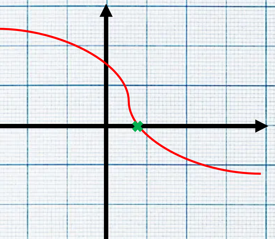
Consider an example where we are trying to find the root of some arbitrary curve shown below. The Y value at our lower bound is clearly closer to our target of zero, so it stands to reason that our solution might actually be closer to that bound than the upper bound. Not always, but it’s a fair guess. Rather than choosing the midpoint, let’s fit a curve between the two points and choose a sample point where it crosses zero.

In the bisection method, the midpoint may have been at X = 0, but our new point is closer to the solution! For longer iterative methods, this improvement in your guess can make a huge difference in algorithm performance. It is important to note that this method will not always improve convergence speed, but oftentimes it does. To find the value of the sample point, there is a very simple formula which can be derived from similar triangles.

Other than the estimate of the sample point, this algorithm is no different than the bisection method. Iterate until your tolerance has been achieved! Let’s modify our code from the bisection method to use the false position method instead. Notice how since the curve we are trying to find a zero for is a straight line, we actually find the solution on the first iteration. Way more efficient!

# False Position Method Python Code Example
# Assume you want to minimize a parabola with the equation y = (1/2) * x^2 + 4
# The derivative is equal to y' = x

# A function to evaluate the derivative (y') at a given x value
def f(x):
    return x
    
# A function to calculate the sample point dervied from similar triangles
def samplePoint(xLower, xUpper):
    return xUpper - (f(xUpper) * (xLower - xUpper)) / (f(xLower) - f(xUpper))
    
# Define Initial Bounds
lowerBound = -3.0
upperBound = 5.0

# Define Convergence Criteria
eps = 1.0e-3

# Loop until the solution is found
i = 0
root = lowerBound # initialize
while (upperBound - lowerBound) > eps:
    # Increment the iteration counter
    i += 1
    
    # Print Iteration Status
    print("Iteration ", i, ", Lower Bound = ", lowerBound, ", upperBound = ", upperBound)
    
    # Estimate the solution
    root = samplePoint(lowerBound, upperBound)

    # Check for an exact solution
    if f(root) == 0.0:
        break
    
    # Check which bound to shift
    # Since we want the new bound to have the same sign as 
    # the one it is replacing, we can say that the product 
    # must be positive
    if f(lowerBound) * f(root) > 0:
        lowerBound = root
    else:
        upperBound = root
        
# Print Solution
print("Found solution at X = ", root)

Conclusion

In today’s post we covered bracketing methods for solving root find problems. The techniques we covered were graphical methods, bisection and false position. I recommend you try to implement these algorithms on your own to solve a problem that interests you.

I hope you enjoyed this post and found the content clear and helpful. Let me know your feedback in the comments or about a project you created using a bracketing method. I hope to see you again soon!

-Parker